System Design for Proximity Service

Problem

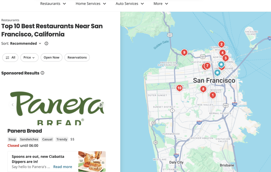
A proximity service enables the discovery of nearby locations, such as restaurants, hotels, theaters, and museums. It serves as a core component for features like finding top-rated restaurants on Yelp or identifying the nearest gas stations on Google Maps, providing users with highly relevant and location-based recommendations.

Requirements

Functional Requirements

We focus on 3 key features:

• Retrieve Businesses: Provide all businesses within a specified radius based on the user’s location (latitude and longitude).
• Manage Businesses: Allow business owners to add, delete, or update their businesses. Real-time updates are not required.
• Business Details: Enable customers to view detailed information about individual businesses.

Non-Functional Requirements

• Low Latency: Users expect immediate results when searching for nearby businesses. The system should deliver responses quickly to enhance user experience and engagement.
• Data Privacy: Location data is highly sensitive, and protecting user privacy is paramount. A location-based service (LBS) must comply with data privacy regulations such as the General Data Protection Regulation (GDPR) and the California Consumer Privacy Act (CCPA). Adopting robust privacy practices ensures user trust and legal compliance.
• High Availability and Scalability: The system should maintain high availability and be capable of scaling to handle traffic surges, particularly during peak hours in densely populated areas, ensuring uninterrupted service and optimal performance.

Back-of-the-envelope Estimation

Assume:

• 100 million daily active users
• 200 million businesses
• Seconds in a day = 24 * 60 * 60 = 86,400
• We can round it up to 10^5 for easier calculation. 10^5 is used throughout this book to represent seconds in a day.
• Assume a user makes 10 search queries per day.
• Search QPS = 100 million * 10 / 10^5 = 10,000
• read:write = 100:1 =>  Read-Heavy System

APIs Design

APIs main:

GET /v1/s/nearby

Field	Description	Type
latitude	Latitude of a given location	decimal
longitude	Longitude of a given location	decimal
radius	Optional. Default is 5000 meters (about 3 miles)	int

Response Body

{
  "total": 20,
  "businesses":[{business object}]
}

Other APIs

APIs	Detail
GET /v1/businesses/{:id}	Detailed information about a business
POST /v1/businesses	Add a business
PUT /v1/businesses/{:id}	Update details of a business
DELETE /v1/businesses/{:id}	Delete a business

Database Design

Columns
Id	bigint
name	string
address	string
city	string
latitude	float
longitude	float

High-Level Design

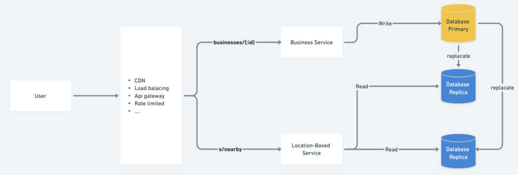
Load Balancer

The load balancer ensures efficient traffic distribution across multiple services. A single DNS entry point is provided, internally routing API calls to the appropriate services based on URL paths.

Location-Based Service (LBS)

The LBS is the core system responsible for finding nearby businesses within a given radius and location. It has the following characteristics:

• Read-Heavy: Primarily handles read requests with minimal or no writes.
• High QPS: Experiences significant traffic, especially during peak hours in densely populated areas.
• Stateless: Easily scalable horizontally to handle varying loads.

Business Service

Handles two main types of requests:

1. Business Management: Business owners can create, update, or delete businesses. These write operations have a low QPS.
2. Customer Queries: Customers view detailed business information, which results in high QPS during peak hours.

Database Cluster

• Uses a primary-secondary setup:
  • The primary database handles write operations.
  • Replicas handle read operations for scalability.
• Data is written to the primary and asynchronously replicated to replicas, which may introduce minor read inconsistencies. This is acceptable as real-time updates are not required for business information.

Scalability

• Both the business service and LBS are stateless, enabling easy horizontal scaling:
  • Peak Hours: Add servers to accommodate traffic (e.g., during mealtimes).
  • Off-Peak Hours: Remove servers to optimize costs.
• Cloud deployment across multiple regions and availability zones enhances scalability and availability.

Detail High-Level Design

Algorithms to fetch nearby businesses

Option 1: Two-dimensional search

SELECT business_id, latitude, longitude
FROM business
WHERE (longitude BETWEEN {:my_long} - radius AND {:my_long} + radius) 
AND (latitude BETWEEN {:my_lat} - radius AND {:my_lat} + radius)
      

Challenges with the Provided Query

1. Table Scans for Large Ranges:
   • The query performs range scans for latitude and longitude separately, which can return large intermediate datasets, especially for a dense area.
   • The database engine must intersect these datasets to determine results within the bounding box, which is computationally expensive.
2. Bounding Box Approximation:
   • The query defines a bounding box for the radius but does not directly calculate whether each point lies within the actual circle (the true radius). This means additional filtering is needed after retrieving the initial dataset.
3. Inefficiency of B-Tree Indexes:
   • B-tree indexes are linear and not optimized for 2D data. They treat latitude and longitude as independent, missing the spatial relationship between them.

Approach: Basic Database Indexing

1. Initial Optimization

To improve the performance of a geographic query, the simplest step is to create a B-tree index on the latitude and longitude columns. This can help narrow down the search range when working with bounding boxes.


CREATE INDEX idx_latitude_longitude ON businesses (latitude, longitude);

This index allows the database to:

• Quickly filter rows where latitude falls within a specific range.
• Then, filter rows where longitude falls within a specific range.

2. Challenges with B-Tree Indexing

While a B-tree index can improve performance in some cases, it’s not ideal for handling geographic queries for the following reasons:

1. Range Queries Are Not Optimized for Multi-Dimensional Data:
   • A bounding box query involves two independent range conditions:
     • latitude BETWEEN :min_lat AND :max_lat
     • longitude BETWEEN :min_long AND :max_long
   • Each condition may produce large intermediate datasets. The database must then intersect these datasets to determine the final result, which is computationally expensive.
2. Lack of Spatial Awareness:
   • B-tree indexes treat latitude and longitude as independent values.
   • They don’t account for the 2D relationship between points, such as the actual distance between them.
3. Inefficiency in Radius Queries:
   • A radius query requires calculating the distance between points based on their coordinates (e.g., using the Haversine formula or geodesic calculations).
   • B-tree indexes cannot optimize this calculation because they’re designed for 1D data and cannot understand the geometry of geographic relationships.

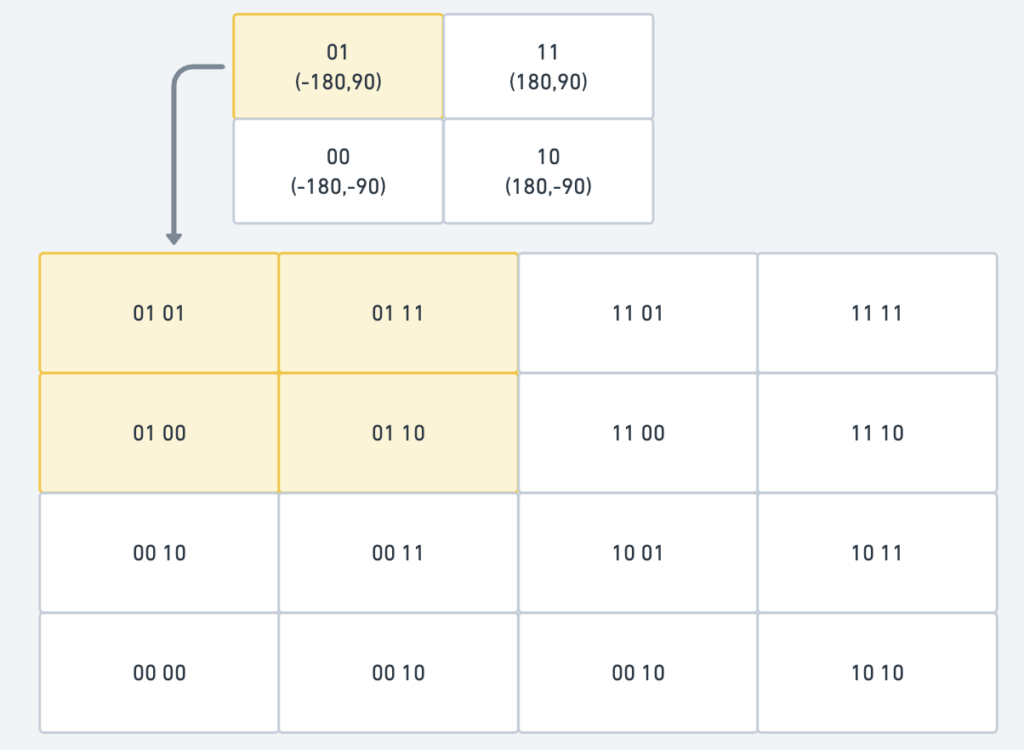
Option 2: Geohash

Geohash is a spatial data encoding technique that converts two-dimensional geographic coordinates (latitude and longitude) into a one-dimensional string of alphanumeric characters. This encoding makes it easier to index and query spatial data while preserving proximity relationships.

First, divide the planet into four quadrants along with the prime meridian and equator.

• The latitude range [-90, 0] is represented by 0
• The latitude range [0, 90] is represented by 1
• The longitude range [-180, 0] is represented by 0
• The longitude range [0, 180] is represented by 1

Second, divide each grid into four smaller grids. Each grid can be represented by alternating between the longitude and latitude bits.

Geohash length	Grid width x height	Use Case
1	5,009.4km x 4,992.6km (the size of the planet)	Continent-level queries
2	1,252.3km x 624.1km	Country-level queries
3	156.5km x 156km	Large region queries
4	39.1km x 19.5km	City-level queries
5	4.9km x 4.9km	Neighborhood-level queries
6	1.2km x 609.4m	Street-level queries
7	152.9m x 152.4m	Building-level queries
8	38.2m x 19m	Room-level queries
9	4.8m x 4.8m	Specific object queries (e.g., cars)
10	1.2m x 59.5cm	Specific object queries (e.g., cars)
11	14.9cm x 14.9cm	Specific object queries (e.g., cars)
12	3.7cm x 1.9cm	Specific object queries (e.g., cars)

Why Geohash Lengths 4–6 Are Optimal

1. Balanced Grid Size:
   • Length < 4: The grid size becomes too large, covering vast areas unsuitable for precise location queries.
   • Length > 6: The grid size becomes too small, leading to excessive granularity and inefficient querying or caching nearby locations.
2. Efficient Radius Queries:
   • Geohashes of length 4–6 provide an ideal balance for querying nearby locations at a city, neighborhood, or street level. This avoids the need to process too many small grids or include overly large areas.
3. Reduced Complexity:
   • We often need to check the target geohash and its neighboring geohashes for radius-based searches. Using a precision of 4–6 limits the number of neighboring grids to a manageable level.
4. Performance vs. Accuracy:
   • These lengths provide sufficient accuracy for most applications (e.g., finding nearby businesses) without overloading the system with unnecessary computations.

Geohash usually uses base32. Let’s take a look at two examples with length = 6.

1001 10110 01001 10001 10000 10111 (base32 in binary) → 9q9jhr (base32)

1001 10110 01001 10000 11011 11010 (base32 in binary) → 9q9hvu (base32)

Boundary issues: Why Close Locations Can Have No Shared Prefix

Geohashes divide the world into a hierarchical grid, but the grid structure follows strict geographic boundaries (e.g., equator and prime meridian). When two locations are near such boundaries, they may fall into entirely different grid regions, leading to geohashes with no shared prefix, despite their close proximity.

Key Example

• France Example:
  • La Roche-Chalais (Geohash: u000) is only ~30 km from Pomerol (Geohash: ezzz).
  • Despite their geographic proximity, they have no shared geohash prefix because they are on opposite sides of a boundary.

Why This Happens

1. Geohash Encoding:
   • Geohashing divides the world into quadrants and sub-quadrants in a hierarchical manner.
   • The prime meridian (0° longitude) and equator (0° latitude) create significant boundaries between quadrants.
   • Locations on opposite sides of these boundaries are encoded with entirely different prefixes.
2. Base32 Representation:
   • Geohashes use Base32 encoding to represent grid cells.
   • Each grid cell belongs to a specific hierarchical region, and boundaries disrupt the continuity of geohash prefixes.

Mitigation Strategies

To address this limitation, combine geohashing with other spatial techniques:

Example:

SELECT * FROM businesses WHERE ST_DWithin(geom, ST_SetSRID(ST_MakePoint(:lon, :lat), 4326)::geography, :radius);

Include Neighboring Geohashes:

• When performing a radius or proximity query, retrieve data not only from the target geohash but also from adjacent geohashes.Use a geohash library to calculate neighbors efficiently.

Example: For u000, include neighbors like u001, ezzz, etc., in the query

SELECT * FROM businesses WHERE geohash IN (:target_geohash, :neighbor_geohash1, :neighbor_geohash2, ...);

Use Bounding Boxes:

Calculate a bounding box for the radius query and filter points based on latitude and longitude.

Refine the results using distance formulas (e.g., Haversine) to ensure accuracy.

Hybrid Approaches:

Combine geohashing with spatial indexes like R-trees or use a database with native spatial support (e.g., PostGIS, MongoDB).

Boundary issue 2

Problem

A second boundary issue arises when:

• Two locations have a long shared geohash prefix, indicating proximity.
• However, they belong to different geohashes due to being on opposite sides of a grid boundary.

Solution

To address this, fetch businesses not only from the target grid but also from neighboring grids:

• Neighboring Geohashes: Neighboring geohashes can be calculated in constant time using geohash libraries. These libraries provide functions to determine adjacent geohashes in all directions (north, south, east, west, and diagonal neighbors).
• Query: SELECT * FROM businesses WHERE geohash IN (:target_geohash, :neighbor_geohash1, :neighbor_geohash2, ...);
  • This ensures businesses near the boundary are included in the results.

Handling “Not Enough Businesses”

When the number of businesses retrieved from the target grid and its neighbors is insufficient, consider the following options:

Option 1: Return Results Only Within the Radius

• Description: Restrict results strictly to businesses within the user-specified radius.
• Advantages:
  • Simple to implement.
  • Guarantees results are strictly within the defined range.
• Disadvantages:
  • May leave the user with too few results, especially in areas with low business density.

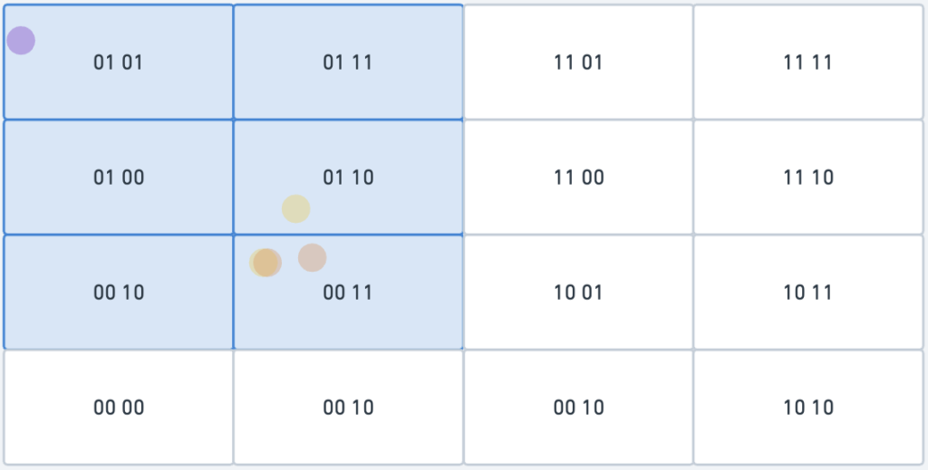
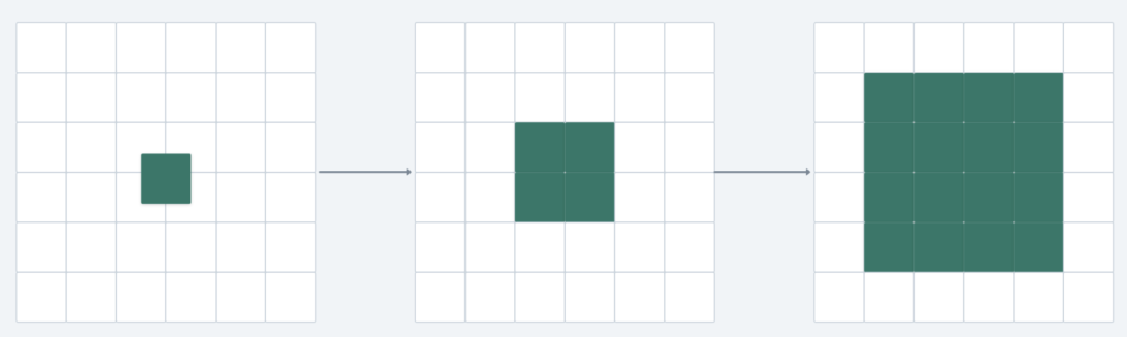
Option 2: Expand the Search Radius Dynamically

• Description: Gradually expand the search area by removing the last digit(s) of the geohash, effectively increasing the grid size.
  • Step 1: Start with the target geohash and its neighbors.
  • Step 2: If the number of businesses is insufficient, remove the last digit of the geohash to expand the grid.
  • Step 3: Repeat until the desired number of results is retrieved or a maximum limit is reached.
• Concept:
  • Removing a digit from the geohash enlarges the search grid hierarchically.
  • This expansion is illustrated in below where the scope grows outward.
• Advantages:
  • Ensures enough results are returned to satisfy user needs.
  • Dynamically adjusts to low-density regions.
• Disadvantages:
  • Expanding the search area too much may include irrelevant results, especially in sparsely populated areas.
  • Query execution time may increase with repeated expansions.

Best Practice

Continue expanding until the result set meets the desired size or a maximum search limit is reached.

Hybrid Approach:

Combine Option 1 and Option 2.

• Start with results strictly within the user-defined radius (Option 1).
• If the results are insufficient, dynamically expand the search area using geohash truncation (Option 2).

Implementation Steps:

• Fetch businesses within the target geohash and its neighbors.
• If the number of results is less than the desired count:
  • Remove the last geohash digit and repeat the query with the expanded grid.
• Continue expanding until the result set meets the desired size or a maximum search limit is reached.

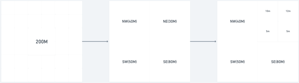
Option 3: Quadtree

A quadtree is a data structure used for partitioning two-dimensional space. It works by recursively subdividing the space into four quadrants (grids) until each grid satisfies a specified criterion. This makes it a highly effective tool for optimizing geographic queries in a Location-Based Service (LBS).

Note that quadtree is an in-memory data structure and it is not a database solution.

How a Quadtree Works

1. Initial Subdivision:
   • The entire world is represented as a single grid (root node).
   • If the grid contains more than the specified number of businesses (e.g., 100), it is subdivided into four equal quadrants.
2. Recursive Subdivision:
   • Each quadrant is checked:
     • If the number of businesses exceeds the threshold (e.g., 100), it is further subdivided into four smaller quadrants.
     • If the number of businesses is within the threshold, subdivision stops.
3. Result:
   • The world is partitioned into grids of varying sizes, with smaller grids in dense areas and larger grids in sparse areas.

Advantages

1. Efficient Query Performance:
   • Reduces the search space by traversing only relevant quadrants.
   • Avoids scanning unrelated areas, improving query speed.
2. Adaptive to Density:
   • Automatically adjusts grid size based on the density of businesses.
3. Lightweight and Fast:
   • As an in-memory structure, it offers near-instantaneous lookups.
4. Flexible Threshold:
   • The subdivision criterion (e.g., 100 businesses per grid) can be adjusted to meet specific business needs.

Challenges

1. Memory Usage:
   • The quadtree must be rebuilt at server start-up, requiring sufficient memory to load all business data.
2. Rebuild Overhead:
   • Any updates to the dataset (e.g., adding or deleting businesses) require rebuilding the quadtree, which can be time-consuming.
3. Not a Database Solution:
   • The quadtree is an in-memory solution and doesn’t replace a database. It complements the database by providing a fast querying layer.

Now that we know the data structure for each node, let’s take a look at the memory usage.

• Each grid can store a maximal of 100 businesses
• Number of leaf nodes = ~300 million / 100 = ~3 million
• Number of internal nodes = 3 million * 1/3 = 1.0 million. If you do not know why the number of internal nodes is one-third of the leaf nodes, please read the reference material.
• Total memory requirement = 2 million * 832 bytes + 1 million * 64 bytes = ~2.0 GB. Even if we add some overhead to build the tree, the memory requirement to build the tree is quite small.

Building the Quadtree

• Time Complexity:O(N/100⋅log⁡(N/100))
  • N: Total number of businesses.
  • N/100​: Approximate number of leaf nodes, assuming 100 businesses per grid.
• Example for 300 Million Businesses:
  • Number of leaf nodes: 300 million/100 = 3 million
  • Logarithmic factor: log⁡(3 million) ≈ 31
  • Total operations: 2 million⋅31 = 62 million steps.
  • Depending on the hardware, this could take a few minutes.
• Key Point:
  • While building the quadtree is computationally intensive, it only occurs during server startup.

Querying Nearby Businesses

• Search Process:
  1. Start at the root node of the quadtree.
  2. Traverse the tree to find the leaf node containing the search origin (e.g., user’s location).
  3. Return businesses from the leaf node if it has enough businesses (e.g., 100).
  4. If not, fetch businesses from neighboring nodes until the desired number of results is achieved.
• Key Advantage:
  • The quadtree structure minimizes the search space, making queries fast by focusing only on relevant quadrants.

Operational Considerations

a. Server Start-Up Time

• Building the quadtree may take several minutes, during which the server is unable to handle traffic.
• Mitigation Strategies:
  1. Incremental Rollout:
     • Deploy the new quadtree index to a small subset of servers at a time.
     • Gradually replace servers in the cluster, avoiding widespread downtime.
  2. Blue/Green Deployment:
     • Build the quadtree on a separate cluster.
     • Once ready, switch traffic to the new cluster.
     • Caution: If all servers in the new cluster simultaneously query the database for 300 million businesses, it could overload the system.

b. Updating the Quadtree

1. Nightly Rebuild:
   • Rebuild the quadtree at regular intervals (e.g., every night).
   • Use a business agreement where new or updated businesses become effective the next day.
   • Trade-Off: Some servers may serve stale data temporarily.
   • Challenge: Invalidating a large number of cache keys at the same time can strain cache servers.
2. On-the-Fly Updates:
   • Dynamically update the quadtree as businesses are added or removed.
   • Complexity:
     • Requires thread-safe mechanisms to handle concurrent updates.
     • Locking mechanisms can degrade performance and complicate the implementation.
3. Hybrid Approach:
   • Combine nightly rebuilds with limited real-time updates for critical changes (e.g., high-priority business updates).

Main Factors: Geohash vs Quadtree

Factor	Geohash	Quadtree
Ease of Implementation	Simple; no tree-building required.	More complex; requires tree construction.
Radius Queries	Works well but struggles with dynamic grid adjustments.	Handles radius queries but excels in k-nearest searches.
K-Nearest Queries	Requires additional logic for k-nearest.	Naturally supports k-nearest queries.
Dynamic Grid Size	Fixed grid size; not density-aware.	Automatically adjusts grid size based on density.
Update Complexity	Easy; direct row updates in constant time.	Complex; requires tree traversal and potential rebalancing.
Memory Usage	Minimal; database column storage only.	Higher; requires in-memory tree (~2.0 GB for 300M businesses).
Concurrency	Thread-safe and simple.	Requires locking mechanisms for thread safety during updates.
Effective	Simple	Detail

Option 4: Elasticsearch

Geospatial Index: Elasticsearch supports geohashing, quadtrees, and R-trees for efficient spatial queries.

Example Query: Businesses within a 10km radius of a given location.

Advantages of Elasticsearch

1. Multi-Faceted Search:
   • Combines geospatial, full-text, and categorical filters in a single query.
   • Returns ranked results based on relevance.
2. Performance:
   • Optimized for high-speed queries over large datasets.
   • Handles complex query logic better than traditional relational databases.
3. Scalability:
   • Distributed architecture enables horizontal scaling across nodes.
4. Flexibility:
   • Supports various indexing strategies and custom scoring mechanisms.

Challenges with Elasticsearch

Not a Primary Database

• Elasticsearch lacks ACID compliance, making it unsuitable for transactional data storage.
• Solution: Use Elasticsearch as a secondary index, keeping it in sync with a primary database.

Data Synchronization

• Ensuring Elasticsearch stays up-to-date with the primary database is crucial.
• Solution: Use a Change Data Capture (CDC) system:
  • Capture database changes as events.
  • Write these events to a queue or stream (e.g., Kafka).
  • Use a consumer process to apply changes to Elasticsearch.

Fault Tolerance

• Node or network failures can lead to potential data loss if not properly configured.
• Solution:
  • Carefully configure replicas and shard allocation.
  • Regularly back up Elasticsearch data.

Option 5: Postgres with extension

PostGIS:

• Enables geospatial data support in PostgreSQL.
• Allows indexing and querying of geographic data like latitude and longitude.
• Example: Searching businesses within a given radius.

Command to Enable:

CREATE EXTENSION IF NOT EXISTS postgis;

pg_trgm:

• Supports full-text search using trigram-based indexing.
• Allows fast, fuzzy, or approximate matching for text fields (e.g., names, descriptions).

Command to Enable:

CREATE EXTENSION IF NOT EXISTS pg_trgm;

Advantages

1. Consistency:
   • No need for a separate service (like Elasticsearch); data remains consistent within PostgreSQL.
   • Avoids synchronization issues between a primary database and a search engine.
2. All-in-One Solution:
   • Combines geospatial and full-text search within a single database.
   • Simplifies the architecture.
3. Scalability for Moderate Data Sizes:
   • Handles datasets like 10M businesses (~10GB) and 1TB of reviews without issues.
4. Ease of Maintenance:
   • Reduces operational complexity by avoiding multiple services.

Challenges

1. Full-Text Search Performance:
   • While pg_trgm is efficient for text search, it may not perform as well as Elasticsearch for very large datasets or complex text queries.
2. Scaling:
   • PostgreSQL can handle moderate-scale datasets (e.g., 1TB), but Elasticsearch is better suited for very large-scale data with high read/write demands.
3. Operational Overhead:
   • Managing large indexes (e.g., spatial or full-text) within PostgreSQL requires careful tuning and periodic maintenance (e.g., vacuuming and reindexing).

Geospatial index table
Scaling the Geospatial Index Table

Geohash Indexing

• Two Structuring Options:
  • Option 1: Store all business IDs for a geohash in a single row as a JSON array.
  • Option 2: Store each business ID in a separate row with a compound key of (geohash, business_id).

Recommendation: Option 2

Why?

Option 2 eliminates the need for locking because rows are independently updated.

Ease of Updates:

In Option 1:

Updating a business requires fetching the JSON array, scanning it for the relevant ID, and modifying it.

This process requires locking the row to prevent concurrent updates, adding complexity.

In Option 2:

Updating a business is as simple as inserting, deleting, or updating a single row. No complex locking or array scanning is needed.

Insertions:

In Option 1:

Adding a new business requires scanning the array to ensure no duplicates exist.

In Option 2:

Adding a business is a single-row insert operation with no need for duplicate checks, as the compound key enforces uniqueness.

Scalability:

Option 2 scales better for large datasets because operations are row-based rather than dependent on scanning potentially large arrays.

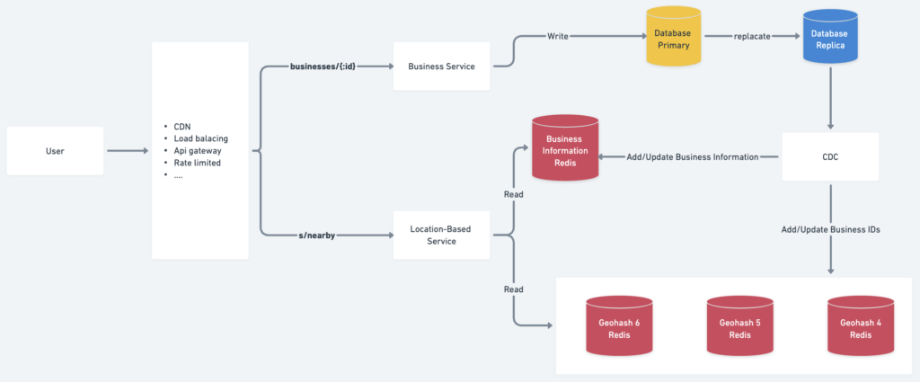
Improve Performance Read Operation

Add Cache

Using caching to improve query performance with geohashes of varying lengths (6, 5, and 4) and precise matching (= instead of LIKE) is an efficient approach. Here’s how this can be structured:

We can add 4 caches:

• Business information:
  • 120: {"name": "Bus", "country": "VN"}
• Geohash Length 6
  • "9q3ynf": [10, 20, 30, 40]
• Geohash Length 5
  • "9q3yn": [10, 20, 30, 40]
• Geohash Length 4
  • "9q3y": [10, 20, 30, 40]

Limitations

1. Cache Consistency:
   • Requires careful synchronization with the database to avoid stale data.
2. Memory Overhead:
   • Maintaining multiple levels of geohash caches can consume significant memory for large datasets.
3. Complexity:
   • Hierarchical fallback logic adds some implementation complexity.

Design diagram

Summary

The Proximity service is a system design, despite its seemingly simple use case, designing it at the internet scale introduces various complex challenges.

References

https://medium.com/@jyoti1308/designing-proximity-service-yelp-7472e1f20cee

https://en.wikipedia.org/wiki/Geohash

https://en.wikipedia.org/wiki/Quadtree